Currently the RAI controller only considers the current market deviation of RAI when deciding system rates. However, the system will benefit from also considering historical error when determing the rate needed to converge market and redemption prices. This is similar to the methodologies of central banks, who examine recent macro-economic indicators when setting interest rates.
Considering historical error will produce stronger rates in time of persistent market deviation(steady state error). This will create stronger incentives for system participants, RAI holders and SAFE Owners, to act and correct the supply/demand imbalance.
To consider historical error, the RAI controller will be switched from a P-only to a PI Controller. The PI Controller is the most common type of closed loop feedback mechanism, used for control of fluid, temperature and even biological systems. Further, research has been shown that some modern monetary policies resemble PI control. (Hawkins et al. 2015)
Calculating the effect of historical error on the rate requires calculating the integral of the error(the sum of the errors in a discrete system). Ki and alpha parameters are then selected to calculate the final contribution of the historical error to the system rate. The Kp parameter is still used to set the current error’s contribution to the rate and will remain unchanged.

Here are the Kp, Ki and alpha(decay) parameters that will be tested on kovan and then deployed to mainnet.

Integral Decay
The error integral is implemented with an alpha parameter that decays the impact of older errors on the controller response. It is a discrete implementation of a leaky integrator
Thus, newer errors are weighted higher than older errors. eg. With a decayed integral, a market deviation from 180 days ago has less effect on the controller response than a market deviation that occurred 7 days ago.
Decaying the error integral also mitigates the risk of any slight bias in the system introduced by code or measurement error. With the decay, this bias will not be able to accumulate forever and ultimately and errantly dominate the rate calculation.
The formula for calculating the error integral is:

In plain language:
“The integral of the error is the time decayed value of the existing integral plus the area of the new error”
Integral Calculation Example

The Effect of Decay
Since the decay of the error only reduces old errors impact and can’t completely eliminate them, we must find an alpha term that approximates the time period we care about.
This is a plot of the cumulative error weight of the new alpha term over a period of 120 days. Notice the weight approaches but doesn’t reach 1. There will still be errors older than 120 days that contribute, albeit very slightly, to the error integral and the controller response.

For the above alpha=0.9999997112,
95% of the error sum occurs within the first 120 days.
5% of the error sum is attributed to errors older than 120 days.
We refer to this as the “120-day alpha”
Definition:
n-day alpha = an alpha that creates a sum where 95% of the sum comes from the most recent n days
Eg. Here is a plot of the 30-day alpha, alpha=0.999998845

The value of alpha determines the age and relative weighting of error(shape of the curve) to use when calculating rates from historical market deviations.
Ki selection
While alpha determines the age of the historical error to use, the Ki parameter determines the magnitude of the rate that comes from the historical error.
When selecting Ki, a major consideration is the length of time it would take for a constant market deviation to double the system rate.
In other words:
“How many days until the rate from the integral equals the rate from the current error?”
equivalently,
“How many days until the Ki rate/Kp rate ratio equals 1?”
For a given Ki, the number of days is dependent upon the alpha parameter.
Given:
Kp=7.5E^-8
Ki=2.4E^-14
alpha=0.9999997112
Table showing the ratios for the new parameters over time for constant error.
| Ki/Kp Rate after 10 days | Ki/Kp Rate after 20 days | Ki/Kp Rate after 30 days | Ki/Kp Rate after 60 days | Ki/Kp Rate after 90 days |
|---|---|---|---|---|
| 0.26 | 0.45 | 0.60 | 0.87 | 1.0 |
As expected, the rate from the integral gets stronger the longer a steady error exists.
Controller Responses
Given these new parameters, here is the new system’s response to step and impulse inputs.
redemption price = 3.0
Kp=7.5E^-8
Ki=2.4E^-14
alpha=0.9999997112
Step Input(Constant Error)
-1% error

-5% error
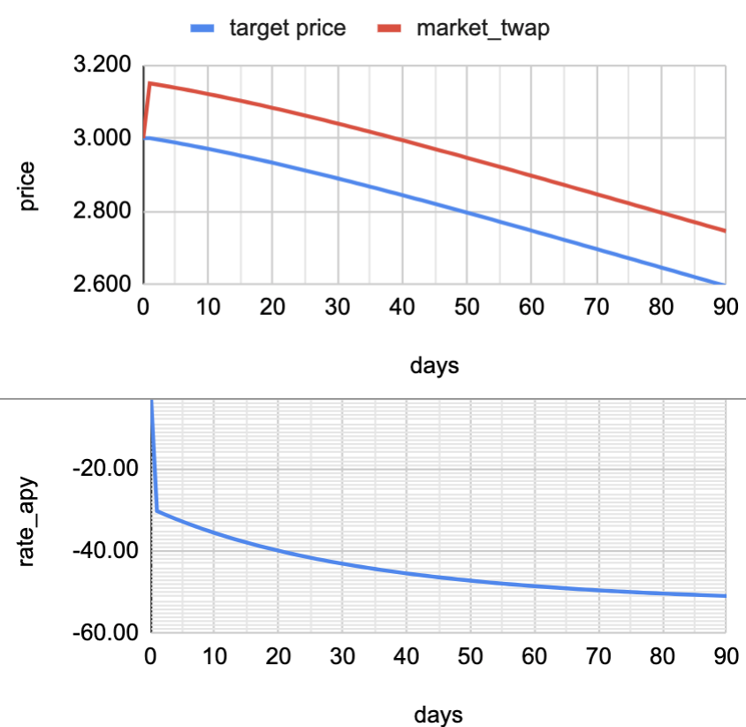
Table of expected systems rates given various levels of constant error(step input) for multiple days. The values for the above plots are bold.
| constant error, $ | constant error, % | annual rate after 30 days | annual rate after 60 days | annual rate after 90 days |
|---|---|---|---|---|
| 0.03 | 1% | 11.9 | 14.2 | 15.3 |
| 0.09 | 3% | 40.1 | 48.8 | 53.1 |
| 0.15 | 5% | 75.4 | 94.0 | 103.4 |
| -0.03 | -1% | -10.6 | -12.4 | -13.2 |
| -0.09 | -3% | -28.6 | -32.8 | -34.7 |
| -0.15 | -5% | -43.0 | -48.4 | -50.8 |
Note: Because of the conversion to APY, the above rates are not symmetrical for positive and negative error. However, the per-second rates in the system are symmetrical and have the same magnitude.
Impulse Input(Instantaneous Error)
-3% impulse

-10% impulse

Table of expected systems rates given various levels of instantaneous error(impulse input). The values for the above plots are bold.
| 1-day impulse error, $ | constant error, % | annual rate after 30 days | annual rate after 60 days | annual rate after 90 days |
|---|---|---|---|---|
| -0.09 | -3% | -0.3 | -0.1 | -0.1 |
| -0.15 | -5% | -0.5 | -0.2 | -0.1 |
| -0.30 | -10% | -1.0 | -0.5 | -0.2 |
| 0.09 | 3% | 0.3 | 0.1 | 0.1 |
| 0.15 | 5% | 0.5 | 0.2 | 0.1 |
| 0.20 | 10% | 1.0 | 0.5 | 0.2 |
Note: Because of the conversion to APY, the above rates are not symmetrical for positive and negative error. However, the per-second rates in the system are symmetrical and have the same magnitude.
References
This is a grid showing step responses for various settings of alpha and Ki for Kp=7.5E^-8.
